Traps

1. Overview

Aquarius allows users to manually specify one or more traps within a device structure. This feature is useful for modelling interface traps, oxide charges, bulk defects, or other non-mobile charges that influence local electrostatics.

Traps can be placed in two types of location:

• Interface traps are located on one or more interfaces (region edges). Densities are per unit area.
• Region traps are distributed throughout the bulk of one or more semiconductor regions. Densities are per unit volume.

Once defined, the charge contribution from the traps is automatically applied to all mesh nodes in the trap's location. During assembly of the Poisson equation, the solver includes this contribution by modifying the local charge density.

The total charge caused by the presence of traps ($Q_{t}$) is added to the right-hand side of Poisson’s equation.

$$\begin{equation} \rho = q(p - n + N_D^+ - N_A^-) + Q_{t} \end{equation}$$

---

The total charge caused by the presence of traps is defined as:

$$\begin{equation} Q_{t} = Q_A + Q_D + Q_f \end{equation}$$

where:

• $Q_A$: Charge due to acceptor-like traps (C/cm² for interface traps, C/cm³ for region traps)
• $Q_D$: Charge due to donor-like traps (C/cm² for interface traps, C/cm³ for region traps)
• $Q_f$: Charge due to fixed charge (C/cm² for interface traps, C/cm³ for region traps)

2. Trap Types

Users can define three types of trap:

1. Fixed Charge
2. Acceptor-like Traps
3. Donor-like Traps

2.1. Fixed Charge

Fixed charge is immobile and constant throughout the simulation. It does not depend on bias or occupancy and is defined by the fixed charge density ($N_f$) specified by the user.

$$\begin{equation} Q_f = q \cdot N_f \end{equation}$$

2.2. Acceptor-like Trap Charge

Acceptor traps are negatively charged when occupied by electrons. The trapped charge depends on the trap density $D_{t}^A(E)$ and its probability of occupation $f_A(E)$, which is computed from the local quasi-Fermi level.

$$\begin{equation} Q_A = -q \int_{E_v}^{E_c} D_{t}^A(E) \, f_A(E) \, dE \end{equation}$$

2.3. Donor-like Trap Charge

Donor traps are positively charged when empty. The trapped charge depends on the trap density $D_{t}^D(E)$ and its occupancy probability $f_D(E)$.

$$\begin{equation} Q_D = +q \int_{E_v}^{E_c} D_{t}^D(E) \, \big(1 - f_D(E)\big) \, dE \end{equation}$$

3. Occupation Probability

Aquarius uses a Fermi-Dirac distribution for trap occupancy, meaning trap occupancy changes smoothly near the local quasi-Fermi level.

$$\begin{equation} f_A(E) = \frac{1}{1 + \exp\big(\frac{E - E_{Fp}}{k_B T}\big)} \end{equation}$$ $$\begin{equation} 1 - f_D(E) = \frac{1}{1 + \exp\big(\frac{E_{Fn} - E}{k_B T}\big)} \end{equation}$$

• Acceptor-like traps are fully occupied if $E<<E_{Fp}$ (hole quasi-Fermi level).
• Donor-like traps are fully empty if $E>>E_{Fn}$ (electron quasi-Fermi level).

4. Usage Instructions

4.1. Interface Traps

In order to add an interface trap, at least one region must be defined. To define a new interface trap:

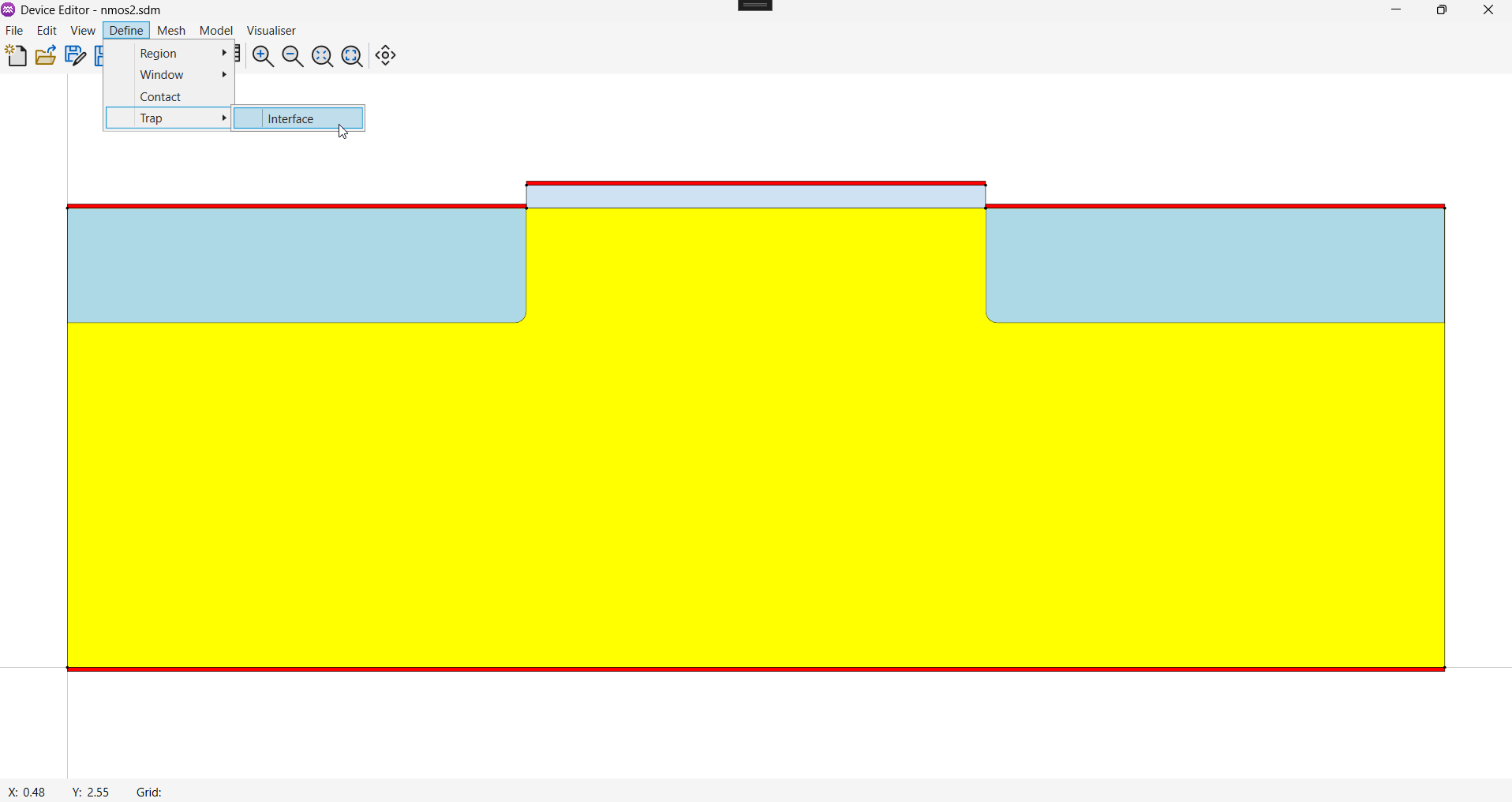
• From the Menu, select Define → Trap → Interface.

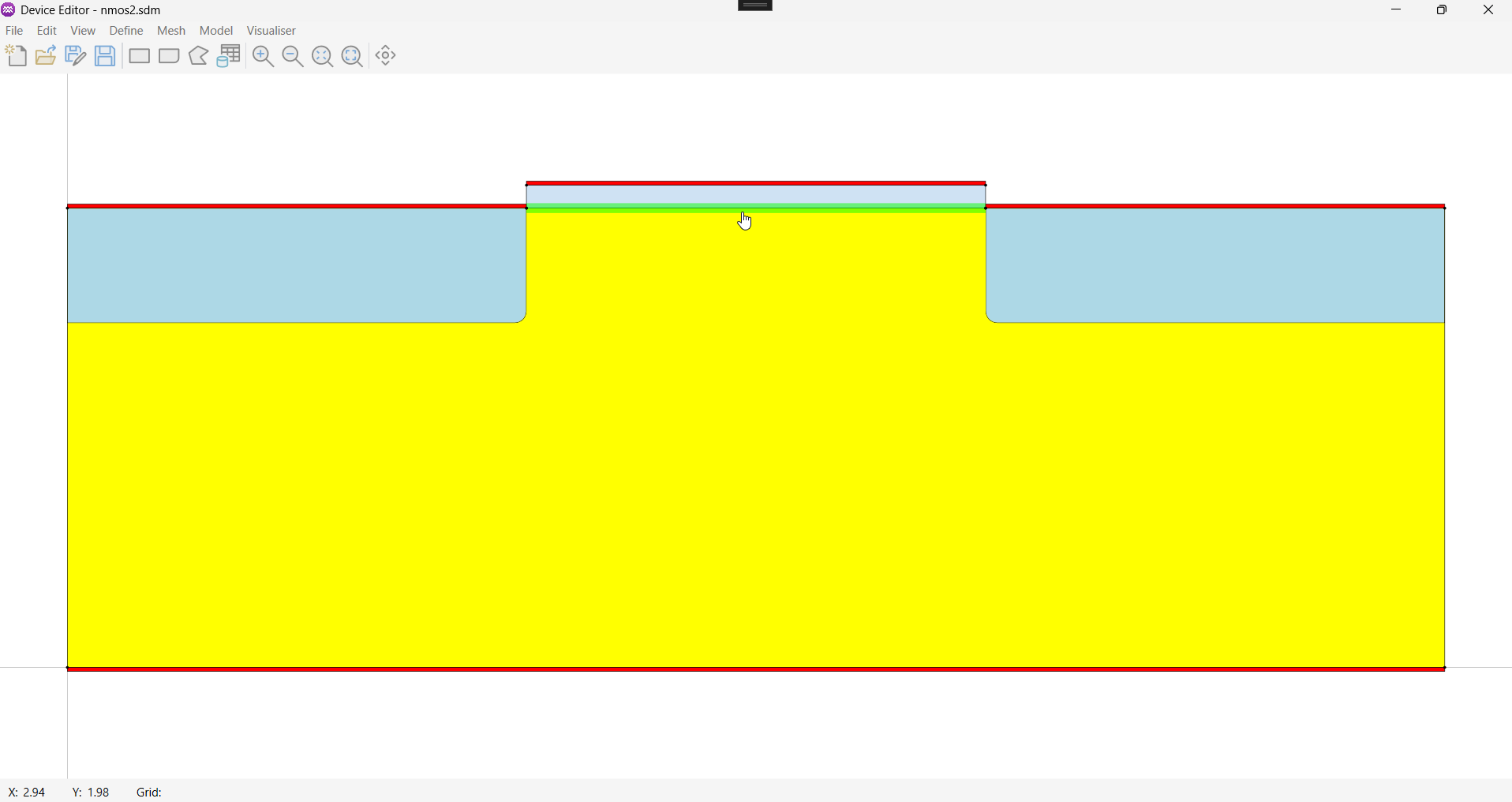
• Using the cursor, hover the cursor over the geometric edges that make up the trap. When the edge is highlighted in green and the cursor changes to indicate a selectable element, left-click to select the edge.

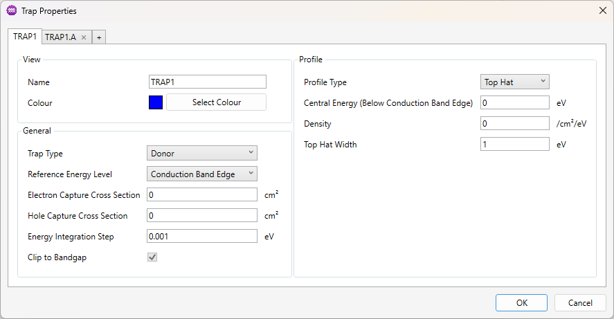
• After selecting all the trap's edges, right-click anywhere to open the properties dialog for the trap. Use this dialog to set the trap's properties.

4.2. Region Traps

In order to add a region trap, at least one semiconductor region must be defined. To define a new region trap:

• From the Menu, select Define → Trap → Region.
• In the Regions section at the top of the properties dialog, tick the regions the trap applies to. Only semiconductor regions are listed. At least one region must be selected.
• Set the trap's properties and click OK. The trap is not added to the device if Cancel is clicked.

Region traps are not drawn on the device canvas. To edit or delete existing region traps, double-click them under Traps in the Device Explorer. Click Delete in the properties dialog to remove the region trap and all of its tabs from the device.

note

Renaming a region automatically updates any region traps that use it. Deleting a region removes it from any region traps, and a region trap is removed from the device if it has no regions left.

4.3. Multiple Traps

Multiple traps can be added to the same location in separate tabs. Click + at the right of the top bar to add a new trap. To delete a trap click the x to the right of its name.

5. Parameters

Densities are per unit area for interface traps and per unit volume for region traps. Where the units differ, the tables below list the unit for each trap type.

5.1. Visual

Name	Description	Unit
Name	A unique identifier for the trap.	-
Colour	Used to define visual colour of the trap. Interface traps only.	-

5.2. General

Name	Description	Unit
Trap Type	Used to define the type of trap. Options: [Fixed, Donor, Acceptor]	-

5.2.1. Fixed

Name	Description	Unit (Interface)	Unit (Region)
Fixed Trap Density	Used to define the density of fixed charges added to the trap location.	cm-2	cm-3

5.2.2. Donor and Acceptor

Name	Description	Unit
Reference Energy Level	Defines the energy level used as reference for the trap energy profile. Options: [Conduction Band Edge, Valence Band Edge, Intrinsic Fermi Level]	-
Hole Capture Cross Section	The effective area of a trap that determines the probability of capturing a hole.	cm2
Electron Capture Cross Section	The effective area of a trap that determines the probability of capturing an electron.	cm2
Energy Integration Level	Used to specify the size of energy level used to approximate the integral across the trap profile.	eV
Clip To Bandgap	If true the density of traps clipped to zero outside the bandgap. Options: [True, False]	-

The capture cross sections are areas for both interface and region traps.

5.3. Profile

Name	Description	Unit
Profile Type	Defines the shape of the trap distribution as a function of energy. Options: [Discrete, Gaussian, Exponential, Top Hat, Table]	-

5.3.1. Discrete

Name	Description	Unit (Interface)	Unit (Region)
Energy Level	The energy for the traps, with respect to the reference energy level.	eV	eV
Density	The concentration of traps per unit area or volume.	/cm2	/cm3

5.3.2. Gaussian

$$\begin{equation} D_{t}(E) = D_0\exp\bigg(\frac{-(E-E_0)^2}{2\sigma^2}\bigg) \end{equation}$$

Name	Description	Unit (Interface)	Unit (Region)
Central Energy	$E_0$ - The midpoint energy for the band of traps, with respect to the reference energy level.	eV	eV
Peak Density	$D_0$ - The concentration of traps per unit area (or volume) and per unit energy at the central energy.	/cm2eV	/cm3eV
Gaussian Sigma	$\sigma$ - The standard deviation of the Gaussian distribution.	eV	eV

5.3.3. Exponential

$$\begin{equation} D_{t}(E) = D_0\exp\bigg(\frac{-|E-E_0|}{E_\text{scale}}\bigg) \end{equation}$$

Name	Description	Unit (Interface)	Unit (Region)
Central Energy	$E_0$ - The midpoint energy for the band of traps, with respect to the reference energy level.	eV	eV
Peak Density	$D_0$ - The concentration of traps per unit area (or volume) and per unit energy at the central energy.	/cm2eV	/cm3eV
Exponential Scale	$E_\text{scale}$ - A parameter controlling the rate of exponential decay.	eV	eV

5.3.4. Top Hat

$$\begin{equation} D_{t}(E) = \begin{cases} D_0, & E_0 - \frac{W}{2} \le E \le E_0 + \frac{W}{2} \\ 0, & \text{Otherwise} \end{cases} \end{equation}$$

Name	Description	Unit (Interface)	Unit (Region)
Central Energy	$E_0$ - Used to specify the midpoint energy for the band of traps, with respect to the reference energy level.	eV	eV
Density	$D_0$ - Used to specify the concentration of traps per unit area (or volume) and per unit energy.	/cm2eV	/cm3eV
Top Hat Width	$W$ - Used to specify the energy range over which traps are uniformly distributed.	eV	eV

5.3.5. Table

A user defined function specified by a list of energy (eV) and density pairs. Density is in /cm²eV for interface traps and /cm³eV for region traps.

The density is linearly interpolated between adjacent energy values and is zero outside the range of energy values provided.